You might have encountered the scenarios where you have to remove table format in Excel. Or maybe you are just reading this article because you are looking for ways to remove completely all the formatting in your table. There are several reasons why you want to remove format in Excel. One of the reasons is because you are preparing data for other users to read and edit the data in their own spreadsheet; another reason is that you need to make things easier when you merge cells.
How to Remove Excel Table Formatting (while keeping the Table)
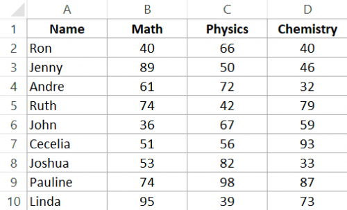
Suppose I have the dataset as shown below.

When I covert this data into an Excel table (keyboard shortcut Control + T), I get something as shown below.https://265ade95220b50a9bdc21686bb8da7b7.safeframe.googlesyndication.com/safeframe/1-0-38/html/container.html

You can see that Excel has gone ahead and applied some formatting to the table (apart from adding filters).
In most cases, I don’t like the formatting Excel automatically applies and I need to change this.
I can now remove the formatting from the table completely or I can modify it to look the way I want.https://265ade95220b50a9bdc21686bb8da7b7.safeframe.googlesyndication.com/safeframe/1-0-38/html/container.html
Let me show you how to do both.
Remove Formatting from the Excel Table
Below are the steps to remove the Excel table formatting:
- Select any cell in the Excel table
- Click the Design tab (this is a contextual tab and only appears when you click any cell in the table)

- In Table Styles, click on the More icon (the one at the bottom of the small scrollbar
- Click on the Clear option.


The above steps would remove the Excel Table formatting, while still keeping it as a table. You will still see the filters that are automatically added, just the formatting has been removed.
You can now format it manually if you want.
Change the Formatting of the Excel Table
If you don’t like the default formatting applied to an Excel Table, you can also modify it by choosing from some presets.
Suppose you have the Excel table and shown below and you want to modify the formatting of this.
Below are the steps to do this:
- Select any cell in the Excel table
- Click the Design tab (this is a contextual tab and only appears when you click any cell in the table)
- In Table Styles, click on the More icon (the one at the bottom of the small scrollbar
- Choose from any of the existing designs

When you hover your cursor over any design, you will be able to see the live preview of how that formatting will look in your Excel Table. Once you have finalized the formatting you want, simply click on it.
In case you don’t like any of the existing Excel table styles, you can also create your own format by clicking on the ‘New Table Styles’. This will open a dialog box where you can set the formatting.
Remove Excel Table (Convert to Range) & the Formatting
It’s easy to convert tabular data into an Excel table, and it’s equally easy to convert an Excel table back to the regular range.
But the thing that can be a bit frustrating is that when you convert an Excel table to the range, it leaves the formatting behind.
And now you have to manually clear the Excel table formatting.
Suppose you have the Excel table as shown below:
Below are the steps to convert this Excel table to a range:
- Right-click on any cell in the Excel table
- Go to the Table option
- Click on ‘Convert to Range’

This will give you a result as shown below (where the table has been deleted but the formatting remains).
Now you can manually change the formatting or you can delete all the formatting altogether.
To remove all the formatting, follow the below steps:
- Select the entire range that has the formatting
- Click the Home tab
- In the Editing group, click on Clear
- In the options that show up, click on Clear Formats
This would leave you with only the data and all the formatting would be removed.
Another way of doing this could be to first remove all the formatting from the Excel Table itself (method covered in the previous section), and then delete the table (Convert to Range).
Delete the Table
This one is easy.
If you want to get rid of the table altogether, follow the below steps:
- Select the entire table
- Hit the Delete key
This will delete the Excel table and also remove any formatting it has (except the formatting that you have applied manually).
In case you have some formatting applied manually that you also want to remove while deleting the table, follow the below steps:
- Select the entire Excel table
- Click the Home tab
- Click on Clear (in Editing group)
- Click on Clear All


Keyboard shortcut to clear all in Excel Windows is ALT + H + E + A (press these keys one after the other in succession).
So these are some scenarios where you can remove table formatting in Excel.
Hope you found this tutorial useful.
Use another method
Excel provides numerous predefined table styles that you can use to quickly format a table. If the predefined table styles don’t meet your needs, you can create and apply a custom table style. Although you can delete only custom table styles, you can remove any predefined table style so that it is no longer applied to a table.

You can further adjust the table formatting by choosing Quick Styles options for table elements, such as Header and Total Rows, First and Last Columns, Banded Rows and Columns, as well as Auto Filtering.
Note: The screen shots in this article were taken in Excel 2016. If you have a different version your view might be slightly different, but unless otherwise noted, the functionality is the same.
Choose a table style
When you have a data range that is not formatted as a table, Excel will automatically convert it to a table when you select a table style. You can also change the format for an existing table by selecting a different format.
- Select any cell within the table, or range of cells you want to format as a table.
- On the Home tab, click Format as Table.
- Click the table style that you want to use.

Notes:
- Auto Preview – Excel will automatically format your data range or table with a preview of any style you select, but will only apply that style if you press Enter or click with the mouse to confirm it. You can scroll through the table formats with the mouse or your keyboard’s arrow keys.
- When you use Format as Table, Excel automatically converts your data range to a table. If you don’t want to work with your data in a table, you can convert the table back to a regular range while keeping the table style formatting that you applied. For more information, see Convert an Excel table to a range of data.
Conclusions
Excel provides three different table styles: the Grid, the Summary and the Data Only. The Data Only style is particularly interesting because Excel removes all formatting – such as borders and shading – and presents your data in a very neat and orderly manner. This is great for making comparisons between two or more sets of data.